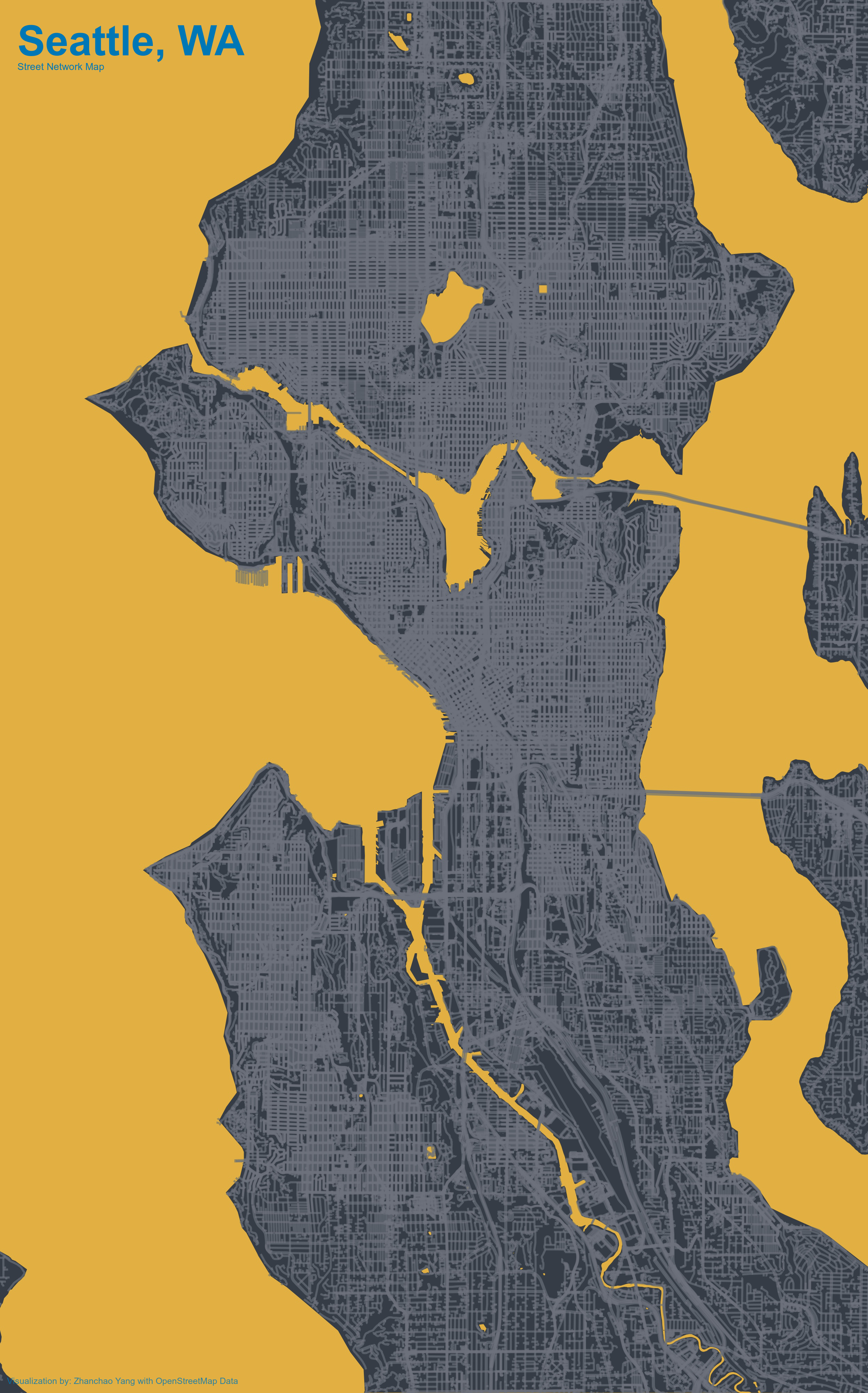
Day 8 (Urban): I created an artistic street network map of Seattle, Washington, visualizing the complex urban fabric through its transportation infrastructure. This map showcases the dense network of highways, primary roads, residential streets, and pathways that define Seattle’s urban landscape. Using OpenStreetMap data, the visualization employs a striking color scheme with a golden yellow background contrasting against dark gray land areas and blue-toned street networks, creating an aesthetically pleasing representation of urban form.
The map focuses on different hierarchies of streets—from major motorways and trunk roads to residential streets, pedestrian paths, and footways—each contributing to the intricate pattern that emerges. Water bodies have been carefully removed from the land area to highlight Seattle’s distinctive geography, bounded by Puget Sound and various lakes.
Acknowledgement:
This visualization was inspired by the tutorial on creating personal art maps by Esteban Moro: Personal art map with R
Technical Implementation:
- osmdata - R package for accessing and querying OpenStreetMap data
- tidyverse - R’s ecosystem of packages for data manipulation and visualization
- sf - R package for handling spatial vector data and geometric operations
- tigris - R package for accessing U.S. Census Bureau TIGER/Line shapefiles (used for county boundaries and water features)
- ggplot2 - R’s powerful data visualization package for creating the map layers
- magick - R package for image processing and annotation
- showtext & sysfonts - R packages for custom font integration (Philosopher font from Google Fonts)
Data Sources:
- Street Network Data: OpenStreetMap - Comprehensive street and highway data for Seattle, including motorways, trunk roads, primary/secondary/tertiary roads, and residential streets
- Administrative Boundaries: U.S. Census Bureau TIGER/Line Shapefiles - County boundaries for Washington State
- Water Features: U.S. Census Bureau Area Water dataset for Washington State counties